| commit | 28e3f07b6336ae154e596be7c7dbb544bfdb6207 | [log] [tgz] |
|---|---|---|
| author | Soumith Chintala <soumith@fb.com> | Sun Nov 06 21:42:49 2016 -0500 |
| committer | Soumith Chintala <soumith@fb.com> | Mon Nov 07 16:17:49 2016 -0500 |
| tree | c1d7242aa80af167b15daf07f256837a3e14ad57 | |
| parent | 513d902df108420dedf3d777738387145998826f [diff] |
adding apply function
| Python | Linux CPU | Linux GPU |
|---|---|---|
| 2.7.8 |  | |
| 2.7 | | |
| 3.3 | | |
| 3.4 | | |
| 3.5 | | |
| Nightly | |
The project is still under active development and is likely to drastically change in short periods of time. We will be announcing API changes and important developments via a newsletter, github issues and post a link to the issues on slack. Please remember that at this stage, this is an invite-only closed alpha, and please don't distribute code further. This is done so that we can control development tightly and rapidly during the initial phases with feedback from you.
PyTorch is a library that consists of the following components:
| _ | _ |
|---|---|
| torch | a Tensor library like NumPy, with strong GPU support |
| torch.autograd | a tape based automatic differentiation library that supports all differentiable Tensor operations in torch |
| torch.nn | a neural networks library deeply integrated with autograd designed for maximum flexibility |
| torch.optim | an optimization package to be used with torch.nn with standard optimization methods such as SGD, RMSProp, LBFGS, Adam etc. |
| torch.multiprocessing | python multiprocessing, but with magical memory sharing of torch Tensors across processes. Useful for data loading and hogwild training. |
| torch.utils | DataLoader, Trainer and other utility functions for convenience |
| torch.legacy(.nn/.optim) | legacy code that has been ported over from torch for backward compatibility reasons |
Usually one uses PyTorch either as:
PyTorch is not a Python binding into a monolothic C++ framework.
It is built to be deeply integrated into Python.
You can use it naturally like you would use numpy / scipy / scikit-learn etc.
You can write your new neural network layers in Python itself, using your favorite libraries.
PyTorch is designed to be intuitive and easy to use.
When you are debugging your program, or receive error messages / stack traces, you are always guaranteed to get error messages that are easy to understand and a stack-trace that points to exactly where your code was defined. Never spend hours debugging your code because of bad stack traces or asynchronous and opaque execution engines.
PyTorch is as fast as the fastest deep learning framework out there. We integrate acceleration frameworks such as Intel MKL and NVIDIA CuDNN for maximum speed.
The memory usage in PyTorch is extremely efficient, and we've written custom memory allocators for the GPU to make sure that your deep learning models are maximally memory efficient. This enables you to train bigger deep learning models than before.
PyTorch is fully powered to efficiently use Multiple GPUs for accelerated deep learning.
We integrate efficient multi-gpu collectives such as NVIDIA NCCL to make sure that you get the maximal Multi-GPU performance.
Writing new neural network modules, or interfacing with PyTorch's Tensor API is a breeze, thanks to an easy to use extension API that is efficient and easy to use.
conda install pytorch -c https://conda.anaconda.org/t/6N-MsQ4WZ7jo/soumith
export CMAKE_PREFIX_PATH=[anaconda root directory]
conda install numpy mkl
conda install -c soumith magma-cuda75# or magma-cuda80
pip install -r requirements.txt
pip install .
Three pointers to get you started:
We will run the alpha releases weekly for 6 weeks. After that, we will reevaluate progress, and if we are ready, we will hit beta-0. If not, we will do another two weeks of alpha.
The beta phases will be leaning more towards working with all of you, convering your use-cases, active development on non-core aspects.
We‘ve decided that it’s time to rewrite/update parts of the old torch API, even if it means losing some of backward compatibility.
This tutorial takes you through the biggest changes and walks you through PyTorch
For brevity,
To reiterate, we recommend that you go through This tutorial
Pickling tensors is supported, but requires making a temporary copy of all data in memory and breaks sharing.
For this reason we're providing torch.load and torch.save, that are free of these problems.
They have the same interfaces as pickle.load (file object) and pickle.dump (serialized object, file object) respectively.
For now the only requirement is that the file should have a fileno method, which returns a file descriptor number (this is already implemented by objects returned by open).
Objects are serialized in a tar archive consisting of four files:
sys_info - protocol version, byte order, long size, etc.pickle - pickled objecttensors - tensor metadatastorages - serialized dataWe made PyTorch to seamlessly integrate with python multiprocessing. What we've added specially in torch.multiprocessing is the seamless ability to efficiently share and send tensors over from one process to another. (technical details of implementation) This is very useful for example in:
Here are a couple of examples for torch.multiprocessing
# loaders.py
# Functions from this file run in the workers

def fill(queue):
  while True:
      tensor = queue.get()
	  tensor.fill_(10)
	  queue.put(tensor)

def fill_pool(tensor):
  tensor.fill_(10)
# Example 1: Using multiple persistent processes and a Queue
# process.py

import torch
import torch.multiprocessing as multiprocessing
from loaders import fill

# torch.multiprocessing.Queue automatically moves Tensor data to shared memory
# So the main process and worker share the data
queue = multiprocessing.Queue()
buffers = [torch.Tensor(2, 2) for i in range(4)]
for b in buffers:
  queue.put(b)
  processes = [multiprocessing.Process(target=fill, args=(queue,)).start() for i in range(10)]
# Example 2: Using a process pool
# pool.py

import torch
from torch.multiprocessing import Pool
from loaders import fill_pool

tensors = [torch.Tensor(2, 2) for i in range(100)]
pool = Pool(10)
pool.map(fill_pool, tensors)
As shown above, structure of the networks is fully defined by control-flow embedded in the code. There are no rigid containers known from Lua. You can put an if in the middle of your model and freely branch depending on any condition you can come up with. All operations are registered in the computational graph history.
There are two main objects that make this possible - variables and functions. They will be denoted as squares and circles respectively.

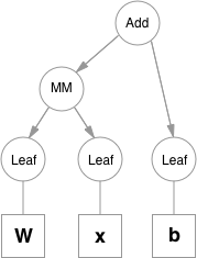
Variables are the objects that hold a reference to a tensor (and optionally to gradient w.r.t. that tensor), and to the function in the computational graph that created it. Variables created explicitly by the user (Variable(tensor)) have a Leaf function node associated with them.

Functions are simple classes that define a function from a tuple of inputs to a tuple of outputs, and a formula for computing gradient w.r.t. it's inputs. Function objects are instantiated to hold references to other functions, and these references allow to reconstruct the history of a computation. An example graph for a linear layer (Wx + b) is shown below.
Please note that function objects never hold references to Variable objects, except for when they're necessary in the backward pass. This allows to free all the unnecessary intermediate values. A good example for this is addition when computing e.g. (y = Wx + My):
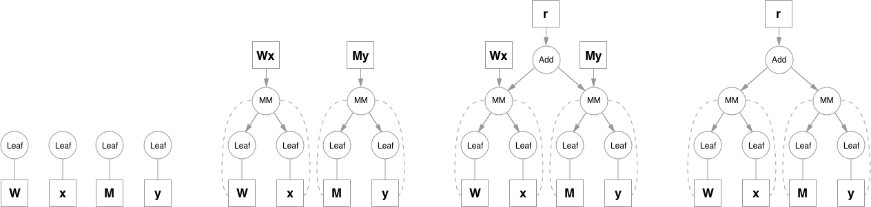
Matrix multiplication operation keeps references to it‘s inputs because it will need them, but addition doesn’t need Wx and My after it computes the result, so as soon as they go out of scope they are freed. To access intermediate values in the forward pass you can either copy them when you still have a reference, or you can use a system of hooks that can be attached to any function. Hooks also allow to access and inspect gradients inside the graph.
Another nice thing about this is that a single layer doesn‘t hold any state other than it’s parameters (all intermediate values are alive as long as the graph references them), so it can be used multiple times before calling backward. This is especially convenient when training RNNs. You can use the same network for all timesteps and the gradients will sum up automatically.
To compute backward pass you can call .backward() on a variable if it‘s a scalar (a 1-element Variable), or you can provide a gradient tensor of matching shape if it’s not. This creates an execution engine object that manages the whole backward pass. It‘s been introduced, so that the code for analyzing the graph and scheduling node processing order is decoupled from other parts, and can be easily replaced. Right now it’s simply processing the nodes in topological order, without any prioritization, but in the future we can implement algorithms and heuristics for scheduling independent nodes on different GPU streams, deciding which branches to compute first, etc.